
Introduction
In this NLP getting started challenge on kaggle, we are given tweets which are classified as 1 if they are about real disasters and 0 if not. The goal is to predict given the text of the tweets and some other metadata about the tweet, if its about a real disaster or not.
In this part 2 for Nearest Neighbor Modelling, I will use the processed data generated in Part 1 to train nearest neighbor models in order to predict if a tweet is about a real disaster or not using the tidymodels framework.
Analysis
Load Libraries
rm(list = ls())
library(tidyverse)
library(ggplot2)
library(tidymodels)
library(silgelib)

theme_set(theme_plex())
Loading processed data from previous part
tweets <- readRDS("../data/nlp_with_disaster_tweets/tweets_proc.rds")
tweets_final <- readRDS("../data/nlp_with_disaster_tweets/tweets_test_proc.rds")
tweets %>%
dim## [1] 7613 830tweets_final %>%
dim## [1] 3263 829Feature preprocessing and engineering
tweets %>%
  mutate(target = as.factor(target),
         id = as.character(id)) -> tweets
tweets %>%
count(target, sort = T)## # A tibble: 2 x 2
## target n
## <fct> <int>
## 1 0 4342
## 2 1 3271Split data
Splitting the data into 3 sets. A test set of 10% data, a cross validation set of 20% data and a training set of 70% data. Training and validation sets will be used for training, tuning and validating performance of models and comparing among them. Test set will only be used for final estimation of the model performance on unknown data.
set.seed(42)
tweets_split <- initial_split(tweets, prop = 0.1, strata = target)

tweets_test <- training(tweets_split)
tweets_train_cv <- testing(tweets_split)

set.seed(42)
tweets_split <- initial_split(tweets_train_cv, prop = 7/9, strata = target)
tweets_train <- training(tweets_split)
tweets_cv <- testing(tweets_split)dim(tweets_train)## [1] 5328 830dim(tweets_cv)## [1] 1522 830dim(tweets_test)## [1] 763 830Preparation Recipe
I will use the recipe package from tidymodels to generate a recipe for data preprocessing and feature engineering.
recipe(target ~ ., data = tweets_train) %>%
  update_role(id, new_role = "ID") %>%
  step_rm(location, keyword) %>%
  step_mutate(len = str_length(text),
              num_hashtags = str_count(text, "#")) %>%
  step_rm(text) %>%
  step_zv(all_numeric(), -all_outcomes()) %>%
  step_normalize(all_numeric(), -all_outcomes())  %>%
  step_pca(all_predictors(), -len, -num_hashtags, threshold = 0.80)-> tweets_recipe
Note above
- We use the training dataset to create the recipe
- We won’t use ‘id’ field as a predictor, only as an identifier.
- For current analysis, we will drop the location and keyword features.
- Creating a length feature to model the tweet length and another feature to store the number of hashtags in the tweet.
- Getting rid of the text field since we have generated all the features from it that we wanted for now.
- Removing all predictors with zero variance.
- Normalizing all features i.e. centering and scaling.
- Adding dimensionality reduction using PCA to keep 80% variance and reduce the number of features while still keeping our custom features.
tweets_prep <- tweets_recipe %>%
  prep(training = tweets_train,
       strings_as_factors = FALSE)
Modelling
Baseline model
I will first create a baseline model to beat. In this case, we can predict randomly in the ratio of target counts and evaluate the model performance accordingly.
tweets_prep %>%
  juice() %>%
  count(target) %>%
  mutate(prob = n/sum(n)) %>%
  pull(prob) -> probs
set.seed(42)
tweets_prep %>%
bake(new_data = tweets_cv) %>%
mutate(predicted_target = as.factor(sample(0:1,
size = nrow(tweets_cv),
prob = probs, replace = T))) %>%
accuracy(target, predicted_target)## # A tibble: 1 x 3
## .metric .estimator .estimate
## <chr> <chr> <dbl>
## 1 accuracy binary 0.512set.seed(42)
tweets_prep %>%
bake(new_data = tweets_cv) %>%
mutate(predicted_target = as.factor(sample(0:1,
size = nrow(tweets_cv),
prob = probs, replace = T))) %>%
f_meas(target, predicted_target)## # A tibble: 1 x 3
## .metric .estimator .estimate
## <chr> <chr> <dbl>
## 1 f_meas binary 0.581Like, we see above, we have a baseline f1 score of 0.5812. We need to build and train a model that beats this baseline.
set.seed(42)
tweets_prep %>%
  bake(new_data = tweets_test) %>%
  mutate(predicted_target = as.factor(sample(0:1,
                                             size = nrow(tweets_test),
                                             prob = probs, replace = T))) %>%
  accuracy(target, predicted_target)
## # A tibble: 1 x 3
## .metric .estimator .estimate
## <chr> <chr> <dbl>
## 1 accuracy binary 0.503set.seed(42)
tweets_prep %>%
bake(new_data = tweets_test) %>%
mutate(predicted_target = as.factor(sample(0:1,
size = nrow(tweets_test),
prob = probs, replace = T))) %>%
f_meas(target, predicted_target)## # A tibble: 1 x 3
## .metric .estimator .estimate
## <chr> <chr> <dbl>
## 1 f_meas binary 0.574Generating submission file
set.seed(42)
tweets_prep %>%
  bake(new_data = tweets_final) %>%
  mutate(target = as.factor(sample(0:1,
                                   size = nrow(tweets_final),
                                   prob = probs, replace = T))) %>%
  select(id, target) %>%
  write_csv("../data/nlp_with_disaster_tweets/submissions/baseline_cvf_57_testf_57.csv")
K-Nearest Neighbor model
Let’s build a basic KNN model with some default number of neighbors to see how the modelling is done in this framework and checkout how the modelling output looks like.
Basic
knn_spec <- nearest_neighbor(neighbors = 3) %>%
  set_engine("kknn") %>%
  set_mode("classification")

wf <- workflow() %>%
  add_recipe(tweets_recipe)
knn_fit <- wf %>%
add_model(knn_spec) %>%
fit(data = tweets_train)
saveRDS(knn_fit, "../data/nlp_with_disaster_tweets/knn/knn_basic_fit.rds")knn_fit <- readRDS("../data/nlp_with_disaster_tweets/knn/knn_basic_fit.rds")
knn_fit %>%
pull_workflow_fit() -> wf_fit
wf_fit$fit$MISCLASS## optimal
## 3 0.3521021The above shows a simple K-nearest neighbors model using the “kknn” engine. Gives about 0.3521021 of minimal misclassification. Let’s try and tune the number of neighbors (k) and see if we can interpret the underlying problem space.
Tuning number of neighbors
Using 5-fold cross validation and values of K going from 1 to 100.
set.seed(1234)
folds <- vfold_cv(tweets_train, strata = target, v = 5, repeats = 1)

tune_spec <- nearest_neighbor(neighbors = tune()) %>%
  set_mode("classification") %>%
  set_engine("kknn")

neighbor_grid <- expand.grid(neighbors = seq(1,100, by = 1))
set.seed(1234)
doParallel::registerDoParallel(cores = parallel::detectCores(logical = FALSE))
knn_grid <- tune_grid(
wf %>% add_model(tune_spec),
resamples = folds,
grid = neighbor_grid,
metrics = metric_set(accuracy, roc_auc, f_meas),
control = control_grid(save_pred = TRUE,
verbose = TRUE)
)
saveRDS(knn_grid, "../data/nlp_with_disaster_tweets/knn/knn_grid.rds")knn_grid <- readRDS("../data/nlp_with_disaster_tweets/knn/knn_grid.rds")
knn_grid %>%
collect_metrics()## # A tibble: 300 x 6
## neighbors .metric .estimator mean n std_err
## <dbl> <chr> <chr> <dbl> <int> <dbl>
## 1 1 accuracy binary 0.628 5 0.00597
## 2 1 f_meas binary 0.705 5 0.00426
## 3 1 roc_auc binary 0.604 5 0.00653
## 4 2 accuracy binary 0.628 5 0.00598
## 5 2 f_meas binary 0.705 5 0.00426
## 6 2 roc_auc binary 0.630 5 0.00928
## 7 3 accuracy binary 0.628 5 0.00544
## 8 3 f_meas binary 0.706 5 0.00349
## 9 3 roc_auc binary 0.639 5 0.00873
## 10 4 accuracy binary 0.628 5 0.00537
## # … with 290 more rowsknn_grid %>%
collect_metrics() %>%
mutate(flexibility = 1/neighbors,
.metric = str_to_title(str_replace_all(.metric, "_", " "))) %>%
ggplot(aes(flexibility, mean, color = .metric)) +
geom_errorbar(aes(ymin = mean - std_err,
ymax = mean + std_err), alpha = 0.5) +
geom_line(size = 1.5) +
facet_wrap(~.metric, scales = "free", nrow = 3) +
scale_x_log10() +
theme(legend.position = "none") +
labs(title = "Model performance against model flexibility",
subtitle = "F1-score peaks around lower flexibility values",
x = "Model flexibility i.e. Log(1/NumberOfNeighbors)",
y = "Mean metric value")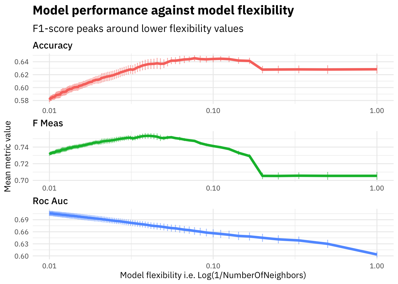
As we see in the plot above, the f1-score increases on the evaluation set until around K=20 and then starts falling down. We plot the flexibility (i.e. 1/NumberOfNeighbors) to visualize how the model performance varies as the model flexibility increases. The KNN model with K=1 will be highly flexible and thus have high variance, whereas K=100 would lead to a much stricter model which is less flexible and might suffer from bias.
Looks like our underlying problem stays much closer to being flexible than strict (since optimal K looks to be around 20). We should remember this fact for picking further models for experimentation.
Let’s pickout the best parameter K based on the highest f1-score and train our final model on the full training dataset and evaluate against cross validation dataset.
knn_grid %>%
  select_best("f_meas") -> highest_f_meas

final_knn <- finalize_workflow(
  wf %>% add_model(tune_spec),
  highest_f_meas
)
last_fit(final_knn,
tweets_split,
metrics = metric_set(accuracy, roc_auc, f_meas)) -> knn_last_fit
saveRDS(knn_last_fit, "../data/nlp_with_disaster_tweets/knn/knn_last_fit.rds")knn_last_fit <- readRDS("../data/nlp_with_disaster_tweets/knn/knn_last_fit.rds")
knn_last_fit %>%
collect_metrics()## # A tibble: 3 x 3
## .metric .estimator .estimate
## <chr> <chr> <dbl>
## 1 accuracy binary 0.643
## 2 f_meas binary 0.756
## 3 roc_auc binary 0.687Our final fit knn model with K=25 gives an f1-score of 0.7560538, which is much higher than our baseline model on the same CV dataset.
Summary
We can hence learn quite a few things about our underlying problem space by using this basic modelling algorithm K-nearest neighbors and use our learning in further model selection and tuning and also generate a fairly robust model that predicts quite effectively as compared to the baseline model.
Also, this tidymodels framework provides a good modelling structure which can be easily reproduced and used to train a variety of models. In the next part of this series, I will work on another classic modelling algorithm, Lasso Regression, where we will also see if we can identify if there any of these features are much more important than the others and if our 2 custom features are useful.
References
- Project Summary Page - NLP with disaster tweets: Summary
- Project Part 1 - NLP with Disaster Tweets: Part 1 Data Preparation
- Lasso Regression using Tidymodels by Julia Silge.
- Introduction to Statistical Learning - Book