What we can learn from Seattle’s bike-counter data: TidyTuesday Apr 02 2019
TidyTuesday
Keywords
DataAnalysis, DataScience, TidyTuesday, Visualizations, Transportation
Introduction
From the article on Seattle Times - “While millions of public dollars are going for bike lanes in Seattle, the city’s data collection on actual bike-lane ridership is scattered and incomplete. Given they’re the best the public can get, here’s what those numbers can tell us about who’s riding where.”
Analysis
Following along the screencast from David Robinson
library(tidyverse)
library(lubridate)
library(scales)
theme_set(theme_light())
bike_traffic_raw <- readr::read_csv("https://raw.githubusercontent.com/rfordatascience/tidytuesday/master/data/2019/2019-04-02/bike_traffic.csv", col_types = cols(bike_count = col_double(), ped_count = col_logical()))
bike_traffic <- bike_traffic_raw %>%
mutate(date = mdy_hms(date)) %>%
filter(bike_count < 2000) %>%
select(-ped_count)
bike_traffic## # A tibble: 509,082 x 4
## date crossing direction bike_count
## <dttm> <chr> <chr> <dbl>
## 1 2014-01-01 00:00:00 Broadway Cycle Track North Of E Uni… North 0
## 2 2014-01-01 01:00:00 Broadway Cycle Track North Of E Uni… North 3
## 3 2014-01-01 02:00:00 Broadway Cycle Track North Of E Uni… North 0
## 4 2014-01-01 03:00:00 Broadway Cycle Track North Of E Uni… North 0
## 5 2014-01-01 04:00:00 Broadway Cycle Track North Of E Uni… North 0
## 6 2014-01-01 05:00:00 Broadway Cycle Track North Of E Uni… North 0
## 7 2014-01-01 06:00:00 Broadway Cycle Track North Of E Uni… North 0
## 8 2014-01-01 07:00:00 Broadway Cycle Track North Of E Uni… North 0
## 9 2014-01-01 08:00:00 Broadway Cycle Track North Of E Uni… North 2
## 10 2014-01-01 09:00:00 Broadway Cycle Track North Of E Uni… North 0
## # … with 509,072 more rowsbike_traffic %>%
count(crossing, direction)## # A tibble: 13 x 3
## crossing direction n
## <chr> <chr> <int>
## 1 39th Ave NE Greenway at NE 62nd St North 38660
## 2 39th Ave NE Greenway at NE 62nd St South 38660
## 3 Broadway Cycle Track North Of E Union St North 44565
## 4 Broadway Cycle Track North Of E Union St South 44565
## 5 Burke Gilman Trail North 42905
## 6 Burke Gilman Trail South 42902
## 7 Elliot Bay Trail North 45234
## 8 Elliot Bay Trail South 45234
## 9 MTS Trail East 45565
## 10 NW 58th St Greenway at 22nd Ave East 44342
## 11 NW 58th St Greenway at 22nd Ave West 44342
## 12 Sealth Trail North 16054
## 13 Sealth Trail South 16054bike_traffic %>%
ggplot(aes(date)) +
geom_histogram() +
facet_wrap(~ crossing)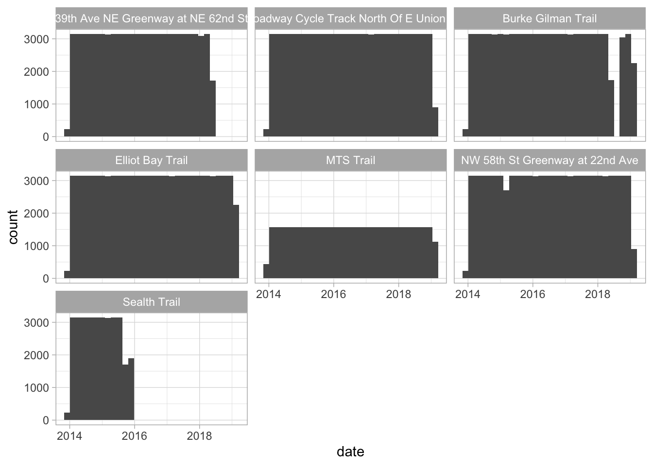
bike_traffic %>%
  ggplot(aes(date)) +
  geom_histogram() +
  facet_grid(crossing ~ direction)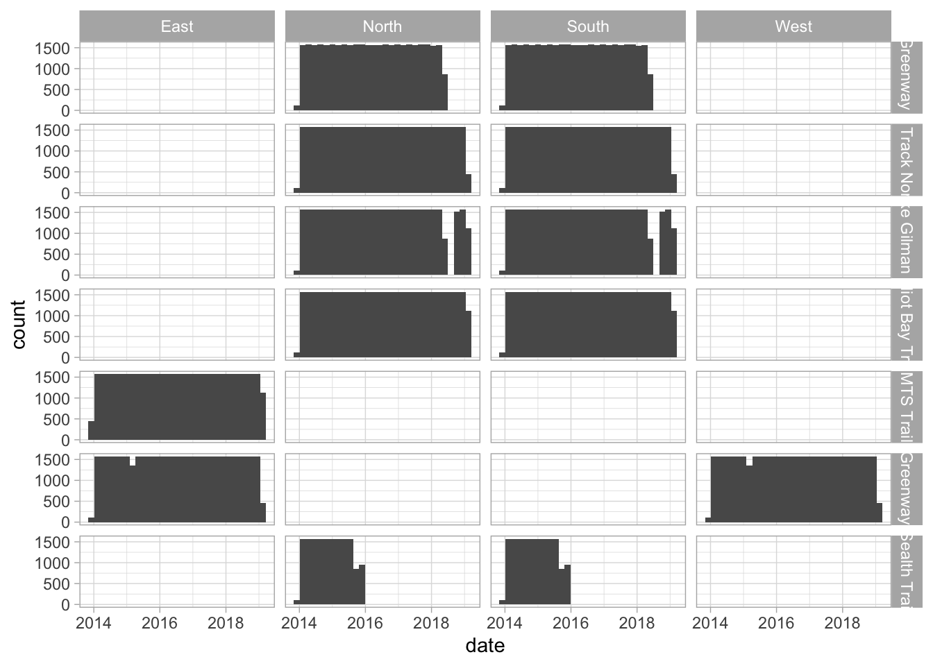
When in the day do we see bikers?
bike_traffic %>%
  group_by(hour = hour(date)) %>%
  summarise(bike_count = sum(bike_count, na.rm = TRUE)) %>%
  ggplot(aes(hour, bike_count)) +
  geom_line() +
  geom_point()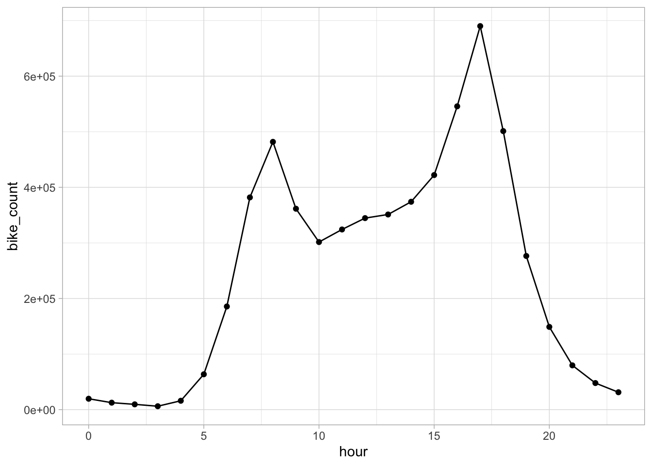
bike_traffic %>%
  group_by(hour = hour(date),
           crossing) %>%
  summarise(bike_count = sum(bike_count, na.rm = TRUE)) %>%
  ggplot(aes(hour, bike_count, color = crossing)) +
  geom_line() +
  geom_point()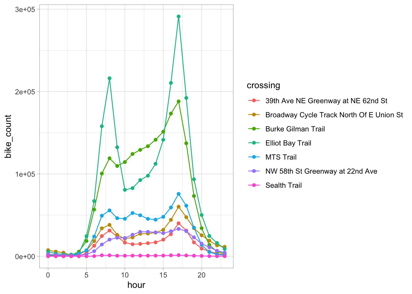
bike_traffic %>%
  group_by(crossing,
           hour = hour(date)) %>%
  summarise(bike_count = sum(bike_count, na.rm = TRUE)) %>%
  mutate(pct_bike = bike_count/sum(bike_count)) %>%
  ggplot(aes(hour, pct_bike, color = crossing)) +
  geom_line() +
  geom_point() +
  scale_y_continuous(labels = percent_format()) +
  labs(title = "When in the day do people bike through these Seattle crossings?",
       subtitle = "Based on crossings from 2014 - Feb 2019",
       color = "Crossing",
       x = "Time of day (local time)",
       y = "% of bike crossings that happen in this hour")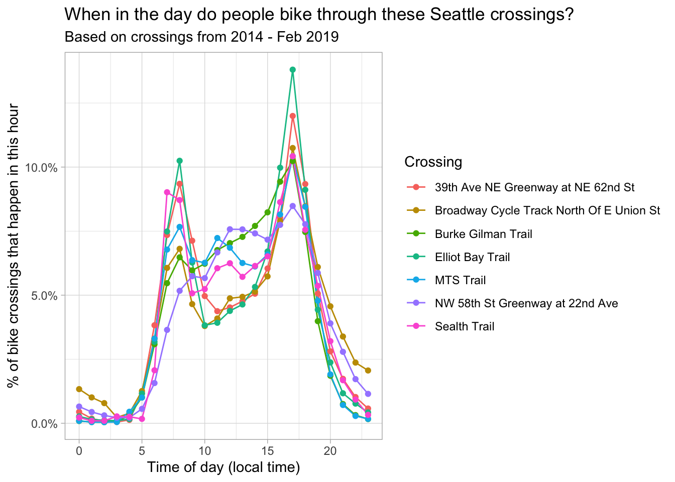
bike_traffic %>%
  mutate(hour = hour(date),
         time_window = case_when(
           between(hour, 7, 10) ~ "Morning Commute",
           between(hour, 11, 15) ~ "Midday",
           between(hour, 16, 18) ~ "Evening Commute",
           TRUE ~ "Night"
         )) %>%
  group_by(crossing,
           time_window) %>%
  summarise(number_missing = sum(is.na(bike_count)),
            bike_count = sum(bike_count, na.rm = TRUE)) %>%
  mutate(pct_bike = bike_count/sum(bike_count)) -> bike_by_time_window

bike_by_time_window %>%
  select(-number_missing, -bike_count) %>%
  spread(time_window, pct_bike) %>%
  mutate(TotalCommute = `Evening Commute` + `Morning Commute`) %>%
  arrange(desc(TotalCommute))
## # A tibble: 7 x 6
## crossing `Evening Commut… Midday `Morning Commut… Night TotalCommute
## <chr> <dbl> <dbl> <dbl> <dbl> <dbl>
## 1 Elliot Bay Trail 0.329 0.250 0.278 0.143 0.607
## 2 39th Ave NE Green… 0.294 0.248 0.288 0.171 0.581
## 3 Sealth Trail 0.266 0.307 0.280 0.147 0.546
## 4 MTS Trail 0.270 0.330 0.271 0.129 0.541
## 5 Burke Gilman Trail 0.271 0.370 0.241 0.117 0.513
## 6 Broadway Cycle Tr… 0.271 0.248 0.213 0.268 0.484
## 7 NW 58th St Greenw… 0.240 0.364 0.202 0.194 0.442bike_by_time_window %>%
ggplot(aes(time_window, pct_bike)) +
geom_col() +
coord_flip() +
facet_wrap(~ crossing)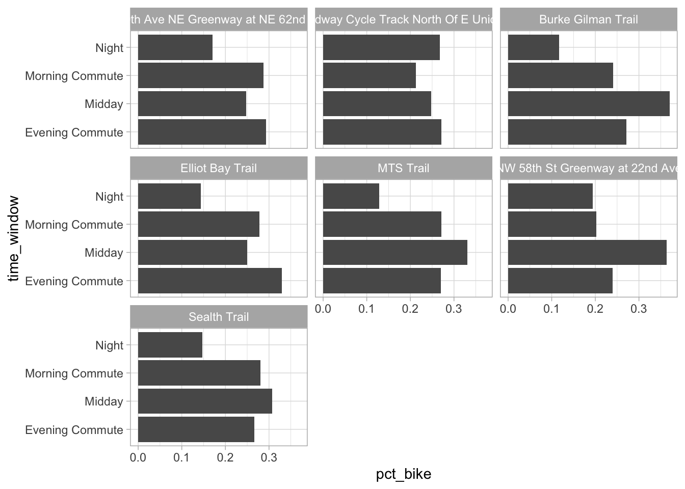
bike_by_time_window %>%
  group_by(crossing) %>%
  summarise(total_bikes = sum(bike_count),
            pct_commute = sum(bike_count[str_detect(time_window, "Commute")]) / total_bikes) %>%
  ggplot(aes(total_bikes, pct_commute)) +
  geom_point() +
  scale_x_log10()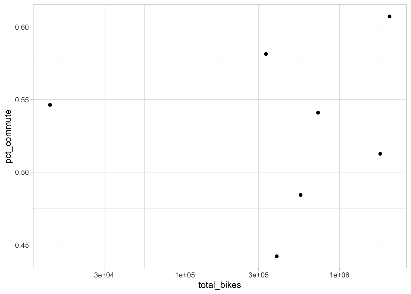
bike_traffic %>%
  group_by(crossing,
           weekday = wday(date, label = TRUE),
        hour = hour(date))  %>%
  summarise(total_bikes = sum(bike_count, na.rm = TRUE)) %>%
  group_by(crossing) %>%
  mutate(pct_bike = total_bikes/sum(total_bikes)) %>%
  ggplot(aes(hour, pct_bike, color = crossing)) +
  geom_line(show.legend = FALSE) +
  facet_grid(crossing ~ weekday) +
  scale_y_continuous(labels = percent_format()) +
  labs(x = "Time of week",
       y = "% of bike crossings happening in this hour",
       title = "When in the week do people in Seattle bike?",
       subtitle = "Based on crossings from 2014-Feb 2019")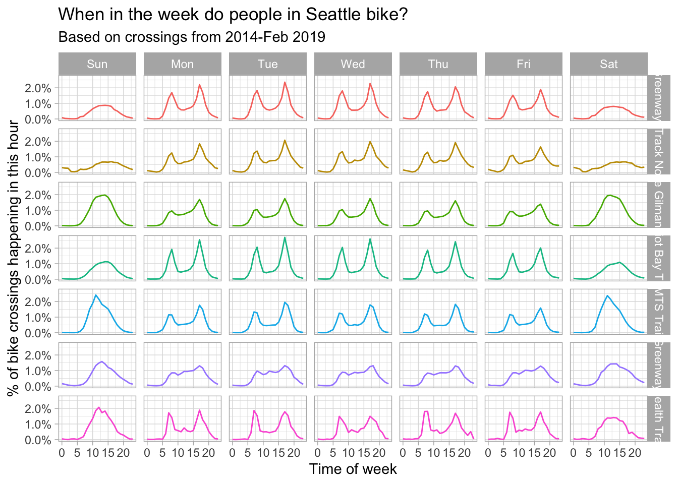
bike_traffic %>%
  filter(date < "2018-01-01") %>%
  group_by(crossing,
           month = fct_relevel(month.name[month(date)], month.name)) %>%
  summarise(total_bikes = sum(bike_count, na.rm = TRUE)) %>%
  mutate(pct_bike = total_bikes/sum(total_bikes)) %>%
  ggplot(aes(month, pct_bike, color = crossing, group = crossing)) +
  geom_line() +
  theme(axis.text.x = element_text(angle = 90, hjust = 1)) +
  expand_limits(y=0) +
  scale_y_continuous(labels = percent_format()) +
  labs(subtitle = "Based on 2014-2017 bike crossings",
       title = "What time of the year did people in Seattle bike?",
       y = "% of yearly trips in this month",
       x = "")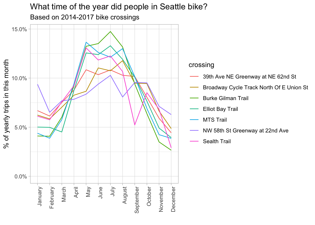
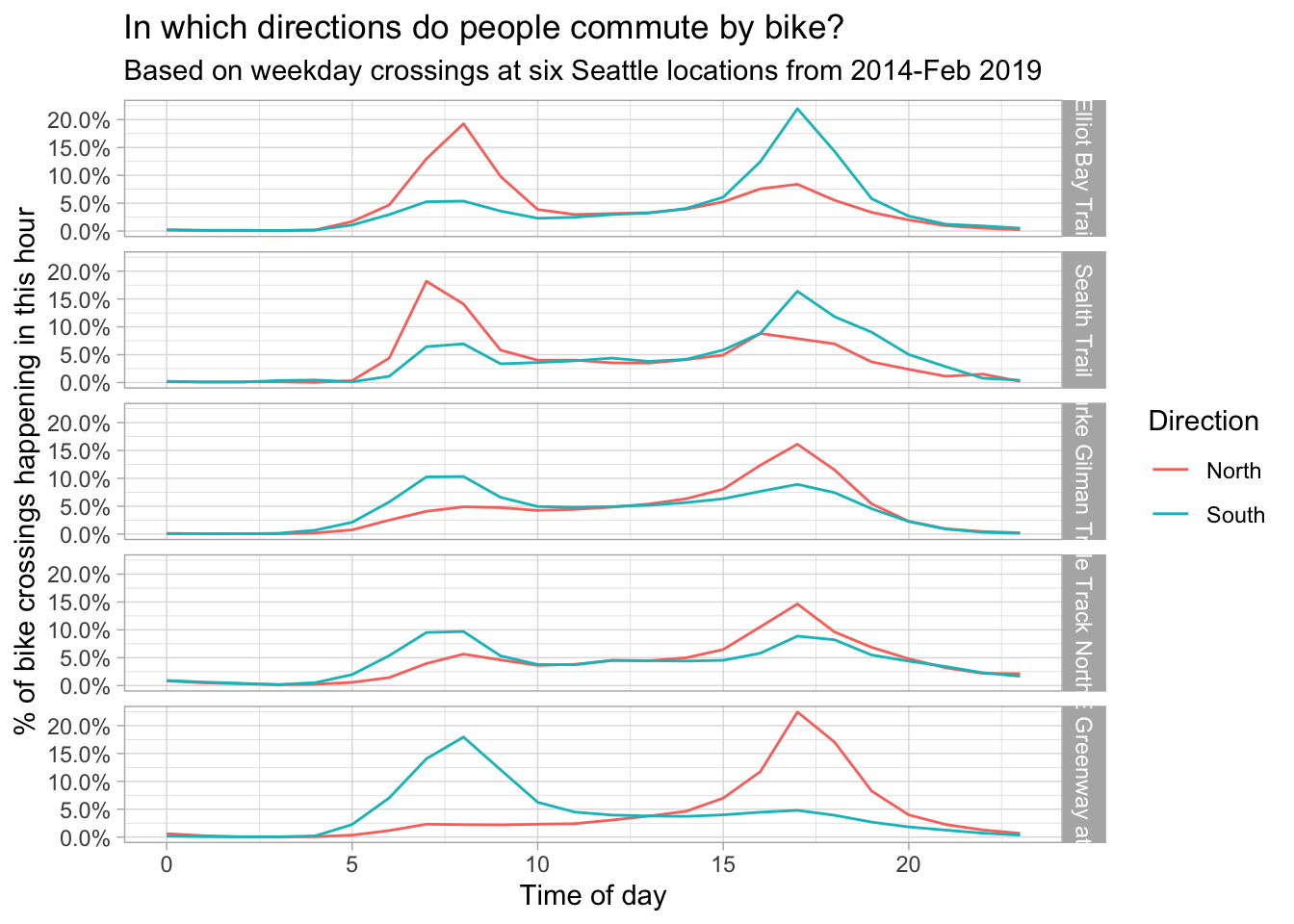
What directions do people commute by bike?
bike_traffic %>%
  filter(crossing != "MTS Trail") %>%
  filter(!wday(date, label = TRUE) %in% c("Sat", "Sun")) %>%
  mutate(hour = hour(date),
         commute = case_when(
           between(hour, 7, 9) ~ "Morning",
           between(hour, 16, 18) ~ "Evening"
         )) %>%
  filter(!is.na(commute)) %>%
  group_by(crossing,
           direction,
           commute) %>%
  summarise(bike_count = sum(bike_count, na.rm = TRUE)) -> bike_by_time_window_commute

bike_by_time_window_commute %>%
  spread(commute, bike_count) %>%
  mutate(ratio = Evening/Morning) %>%
  ggplot(aes(direction, ratio)) +
  geom_col() +
  scale_y_log10(breaks = c(.5, 1, 2, 4, 8),
                labels = c("1/2", "Same", "2x", "4x", "8x")) +
  facet_wrap(~crossing, scales = "free_x")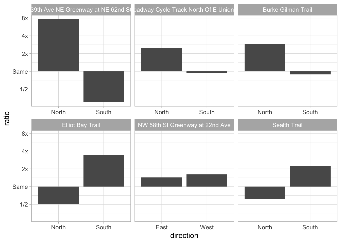
bike_traffic %>%
  filter(crossing != "MTS Trail",
         !wday(date, label = TRUE) %in% c("Sat", "Sun"),
         direction %in% c("North", "South")) %>%
  mutate(hour = hour(date)) %>%
  group_by(crossing,
           direction,
           hour) %>%
  summarise(bike_count = sum(bike_count, na.rm = TRUE)) %>%
  mutate(pct_bike = bike_count/sum(bike_count)) -> bike_by_direction_hour_crossing

bike_by_direction_hour_crossing %>%
  group_by(crossing) %>%
  mutate(average_hour = sum((hour*pct_bike)[direction == "North"])) %>%
  ungroup() %>%
  mutate(crossing = fct_reorder(crossing, average_hour)) %>%
  ggplot(aes(hour, pct_bike, color = direction)) +
  geom_line() +
  facet_grid(crossing ~ .) +
  scale_y_continuous(labels = percent_format()) +
  labs(x = "Time of day",
       y = "% of bike crossings happening in this hour",
       title = "In which directions do people commute by bike?",
       subtitle = "Based on weekday crossings at six Seattle locations from 2014-Feb 2019",
       color = "Direction")