Where Does Your Medicine Come From?: MakeOverMonday 2018 Week 8
tech, DataAnalysis, DataScience, MakeOverMonday, Medicine, Visualizations, R
Introduction
Goal of this Visualization task is to create a visualization for the Drug and Medicine Exports data for different countries. In this blog post, I’m trying to find the leading countries in Export across these 5 years.
Analysis
Cleaning up workspace and loading required libraries
rm(list = ls())library(tidyverse) #Data Wrangling
library("httr")
library(readxl) #Data Ingestion
library(ggplot2) #Data VisualizationObtaining Data
Reading and viewing the dataset
GET("https://query.data.world/s/utmlfljjzc2naoeielefxsf4fh5qkf", write_disk(tf <- tempfile(fileext = ".xlsx")))drugs <- read_excel(tf)drugs## # A tibble: 1,100 x 3
## Exporter Year `Exports (USD)`
## <chr> <dbl> <dbl>
## 1 World 2013 326445385000
## 2 Germany 2013 48493611000
## 3 Switzerland 2013 32337891000
## 4 Belgium 2013 33329615000
## 5 France 2013 27848920000
## 6 United States of America 2013 23098676000
## 7 United Kingdom 2013 20885936000
## 8 Ireland 2013 18152573000
## 9 Italy 2013 20898532000
## 10 Netherlands 2013 13480651000
## # … with 1,090 more rowsSummarizing and getting stats to better understand the dataset
drugs %>%
  glimpse()
## Rows: 1,100
## Columns: 3
## $ Exporter <chr> "World", "Germany", "Switzerland", "Belgium", "France…
## $ Year <dbl> 2013, 2013, 2013, 2013, 2013, 2013, 2013, 2013, 2013,…
## $ `Exports (USD)` <dbl> 326445385000, 48493611000, 32337891000, 33329615000, …drugs %>%
summary()## Exporter Year Exports (USD)
## Length:1100 Min. :2013 Min. :0.000e+00
## Class :character 1st Qu.:2014 1st Qu.:1.212e+05
## Mode :character Median :2015 Median :7.393e+06
## Mean :2015 Mean :3.315e+09
## 3rd Qu.:2016 3rd Qu.:3.293e+08
## Max. :2017 Max. :3.405e+11
## NA's :266Scrubbing data
Removing rows with NA for the purposes of this visualization
drugs = drugs %>%
  filter(!is.na(`Exports (USD)`))
Let’s see overall which are the Countries with highest export over these 5 years.
drugs %>%
  group_by(Exporter) %>%
  summarise(TotalExport = sum(`Exports (USD)`)) %>%
  arrange(desc(TotalExport))
## # A tibble: 220 x 2
## Exporter TotalExport
## <chr> <dbl>
## 1 World 1309425248000
## 2 Germany 197463838000
## 3 Switzerland 183296295000
## 4 France 123482590000
## 5 Belgium 117396245000
## 6 United States of America 114868001000
## 7 United Kingdom 110713945000
## 8 Ireland 96686923000
## 9 Italy 76012918000
## 10 Netherlands 59659401000
## # … with 210 more rowsExploring Data
Lets plot the countries which were among the top 5 exporters each year and each of their performance over these 5 years.
top5ExportersByYear = drugs %>%
  filter(Exporter!="World") %>%
  group_by(Year) %>%
  top_n(5, `Exports (USD)`) %>%
  ungroup()
g = ggplot(data = top5ExportersByYear, aes(x = Year, y = `Exports (USD)`))
g + geom_line(aes(color = Exporter)) + labs(title = 'Trend for top 5 exporters in the world over the years')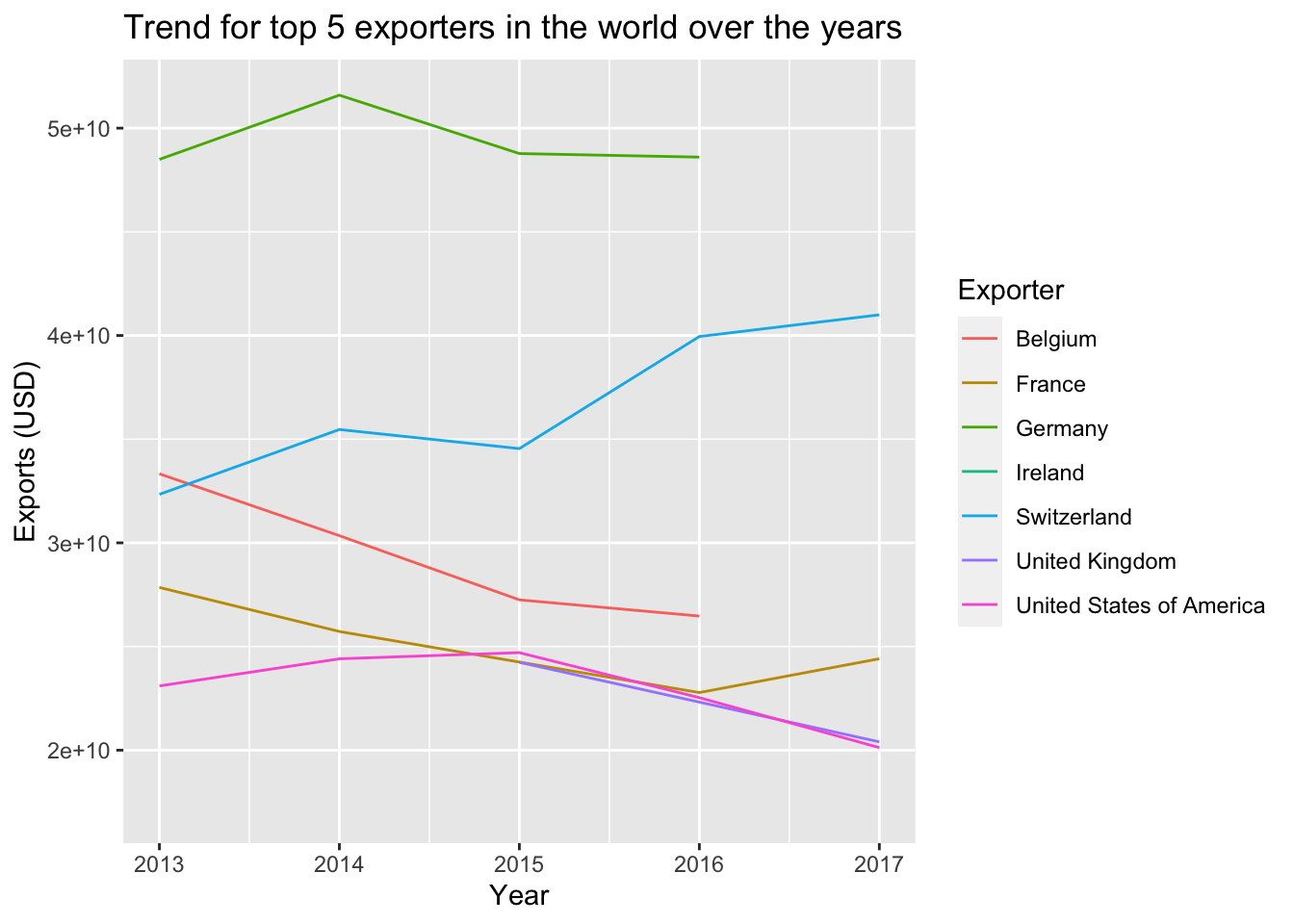 Evaluating Top 10 exporters per Year. Excluding 2017 since we do not have numbers for total export in the world.
getTop10ForYear = function(df){
  top10ForYear = df %>%
    filter(Exporter!="World") %>%
    top_n(10, `Exports (USD)`)

  othersExports = (df %>% filter(Exporter=="World") %>% select(`Exports (USD)`)) - (top10ForYear %>% summarise(Total = sum(`Exports (USD)`)))

  YEAR = df %>% select(Year) %>% unique() %>% .$Year
  top10ForYear = top10ForYear %>%
    add_row(Exporter = "Others", Year = YEAR, `Exports (USD)` = othersExports %>% .$`Exports (USD)`)
  return(top10ForYear)
}
yearlyTop10s = drugs %>%
  filter(Year != 2017) %>%
  group_by(Year) %>%
  do(getTop10ForYear(.))
yearlyTop10s
## # A tibble: 44 x 3
## Exporter Year `Exports (USD)`
## <chr> <dbl> <dbl>
## 1 Germany 2013 48493611000
## 2 Switzerland 2013 32337891000
## 3 Belgium 2013 33329615000
## 4 France 2013 27848920000
## 5 United States of America 2013 23098676000
## 6 United Kingdom 2013 20885936000
## 7 Ireland 2013 18152573000
## 8 Italy 2013 20898532000
## 9 Netherlands 2013 13480651000
## 10 India 2013 10313989000
## # … with 34 more rowsWriting function to plot a Donut Chart for each year showing percentage export contribution for top 10 exporters of that year as compared to all others.
plotTop10 = function(df){
  YEAR = df %>% select(Year) %>% unique() %>% .$Year
  plotTitle = paste("World Medicine Export in", YEAR, sep = " ")

  df = df %>%
    mutate(tot = sum(`Exports (USD)`),
           prop = round(100*`Exports (USD)`/tot,2))

  p = ggplot(df, aes(x=2, y=prop, fill=Exporter)) +
    geom_bar(stat="identity") +
    geom_text( aes(label = prop), position = position_stack(vjust = 0.5)) +
    xlim(0.5, 2.5) +
    coord_polar(theta = "y") +
    labs(x=NULL, y=NULL) +
    labs(fill="") +
    ggtitle(plotTitle) +
    theme_bw() +
    theme(plot.title = element_text(face="bold",family=c("sans"),size=15),
          legend.text=element_text(size=10),
          axis.ticks=element_blank(),
          axis.text=element_blank(),
          axis.title=element_blank(),
          panel.grid=element_blank(),
          panel.border=element_blank())
  return(p)
}
Plotting the donuts for each year
plotTop10(yearlyTop10s %>% filter(Year==2013))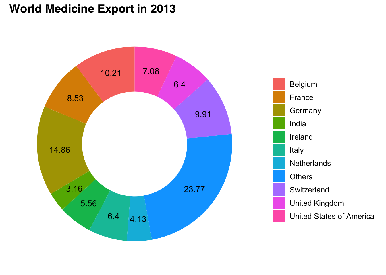
plotTop10(yearlyTop10s %>% filter(Year==2014))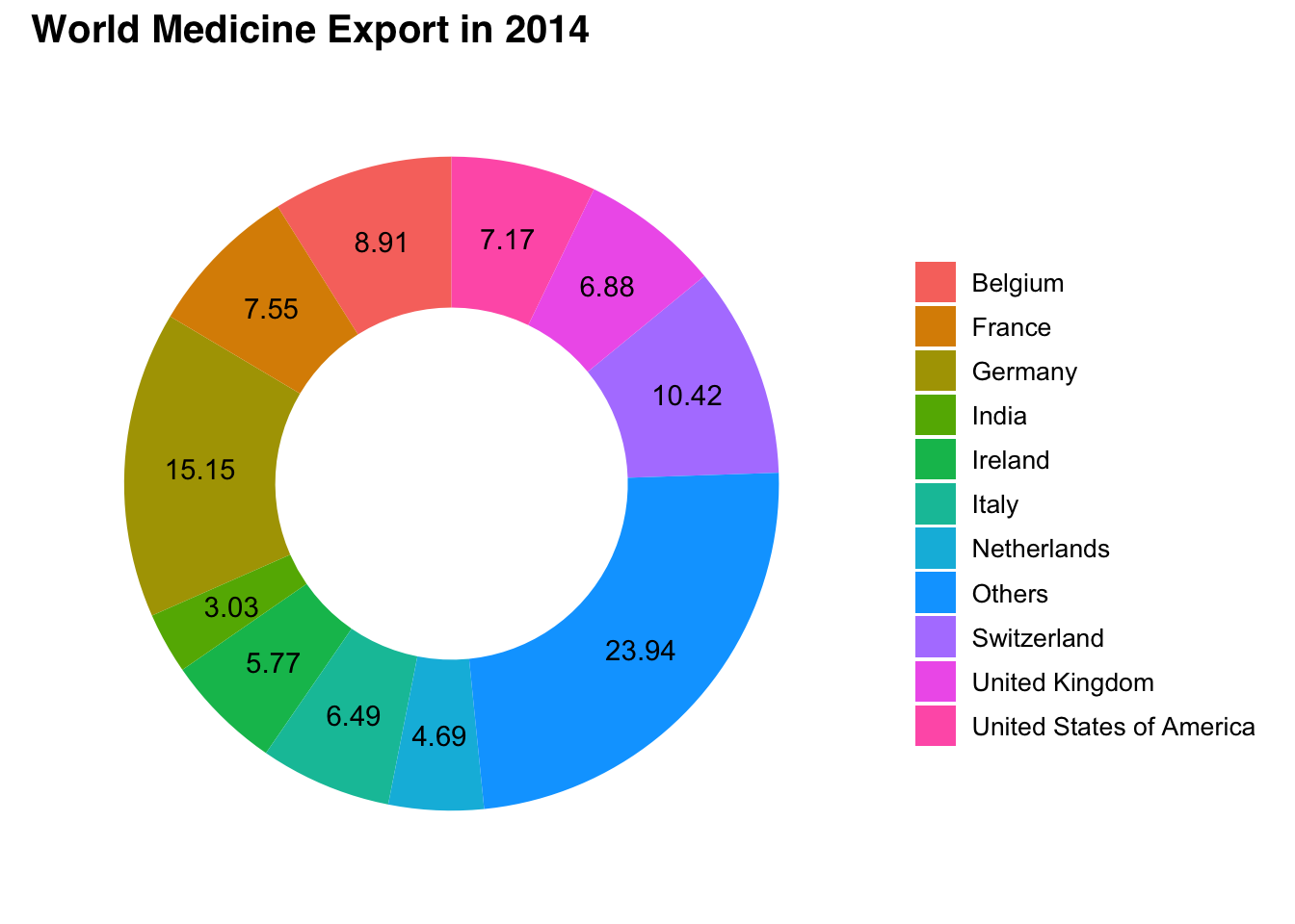
plotTop10(yearlyTop10s %>% filter(Year==2015))
plotTop10(yearlyTop10s %>% filter(Year==2016))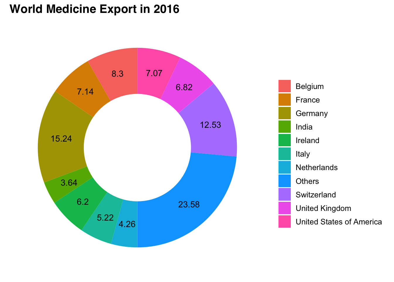 As can be seen Germany remains the biggest exporter of Drugs and Medicines over the past 5 years.